Improving PROTAC properties via single-point changes to linkers
We explore how computational methods can be applied to proteolysis targeting chimera (PROTAC) design, to effectively tackle some of the ...
News
 I am a big fan of the RDKit. In case you have never heard about it, it is an open-source, BSD-licensed C++ toolkit which allows one to accomplish a wide range of cheminformatics tasks. You can build a molecule from SMILES, create 2D depictions, generate 3D conformations, do substructure searches, run chemical reactions, and much more. It comes with C++, Python, Java and C# bindings, so you can access its functionality from your favourite programing language. It features tight integration with the Jupyter notebook, so you can display your molecules in 2D and 3D interactively while you develop your Python workflow. In case you are not much of a programer, a lot of the RDKit functionality is exposed through RDKit KNIME nodes. And, last but not least, the RDKit comes with a PostgreSQL cartridge which enables dealing with molecules in PostgreSQL databases.
Now you know why I love the RDKit, and I hope I managed to convince you to give it a go, if you haven’t already. There are a number of tutorials to get yourself started, and an amazing community of users which can help you out when you are stuck.
Cresset software incorporates the RDKit, which is mostly used to parse SMARTS queries: in Forge, Torch and Spark you may apply SMARTS filters to your molecule tables. In Spark you may also request certain SMARTS patterns to be, or not to be, included in the results; furthermore, the Torsion Library which analyses the torsional angles of the fragments retrieved by a Spark search is based on a database of SMARTS strings.
We also use the RDKit in our internal research projects, in Cresset Discovery Services, and occasionally to integrate or customize the functionality already available in Cresset desktop applications, command-line tools, and KNIME nodes.
Besides being RDKit users, we are also RDKit contributors. In 2015 we contributed a resonance structure enumerator, while at the 2016 RDKit User Group Meeting, which was hosted at the Novartis Campus in Basel, we presented some preliminary work on boosting RDKit molecular simulations through OpenMM.
 OpenMM is an open-source toolkit for high-performance molecular simulations running on CPUs and GPUs. Originally developed in the Pande Lab at Stanford, it is currently supported also by other groups and individuals. OpenMM natively implements AMBER, CHARMM and AMOEBA force fields, which are focused on biological macromolecules, and provides support for implementing custom force fields. The RDKit natively implements MMFF94 and UFF force-fields. MMFF94 is a general-purpose, accurate force-field, while UFF is geared towards small molecules, and trades accuracy for wide chemistry coverage and speed. We thought that it would be interesting to:
Even though OpenMM features outstanding support for custom force fields (it has a lexical parser for energy equations and can even compute their analytical derivatives), MMFF94 has rather complicated combination and scaling rules for non-bonded parameters, which required some tweaking on the OpenMM library to be implemented efficiently. I managed to implement under CPU and GPU platforms the seven energy terms of MMFF94 using a combination of AMOEBA and custom forces:
Below (and on GitHub) you will find a Jupyter notebook showing a geometry optimization benchmark on a small protein, villin.
As you may appreciate going through the notebook, the increase in performance provided by this preliminary proof-of-concept implementation is impressive: OpenMM single and double precision are respectively 150 and 11 times faster than the RDKit implementation on a GeForce GTX 960 graphics card.
Our goal is now to code a native implementation of the MMFF94 and UFF force fields within OpenMM, and then provide the RDKit with an interface to the latter, in order to benefit from the speed-up. Possible applications include the automated minimization of protein-ligand complexes after docking, or the molecular dynamics simulation of small molecules in explicit solvent under periodic boundary conditions. The availability of the latter will be announced on the Cresset website and on the RDKit mailing list.
Here follows the Jupyter Notebook (see it on GitHub):
import sys
import math
import timeit
from rdkit import Chem
from rdkit.Chem import AllChem
from rdkit.Chem import Draw
from rdkit.Chem.Draw import IPythonConsole
import py3Dmol
from simtk.openmm import openmm
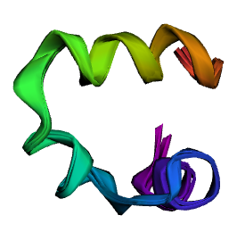
This is the villin headpiece as downloaded from the PDB:
villin = open('/home/paolo/pdb/2F4K.pdb', 'r').read()
p = py3Dmol.view(width = 400,height = 400)
p.addModel(villin, 'pdb')
p.setStyle({'cartoon': {'color':'spectrum'}})
p.zoomTo()
p.show()
molOrig = Chem.MolFromPDBBlock(villin)
mol = Chem.AddHs(molOrig, addCoords = True)
pyMP = AllChem.MMFFGetMoleculeProperties(mol)
pyMP.SetMMFFVariant('MMFF94s')
Let’s create 4 forcefields, the “traditional” one and those spiced up with OpenMM, respectively using single and double precision CUDA kernels, and the multi-threaded single-precision CPU implementation.
for i in range(3):
    mol.AddConformer(Chem.Conformer(mol.GetConformer(0)), assignId = True)
platformNames = ['RDKit', 'OpenMM_CUDA_s', 'OpenMM_CUDA_d', 'OpenMM_CPU']
pyFF = {}
pyFF[platformNames[0]] = AllChem.MMFFGetMoleculeForceField(mol, pyMP, confId = 0)
for i in range(1, 4):
    pyFF[platformNames[i]] = AllChem.MMFFGetMoleculeOpenMMForceField(mol, pyMP, confId = i)
Now we instruct our RDKit interface to OpenMM to use the appropriate hardware platform:
pyFF['OpenMM_CUDA_s'].InitializeContext(
    'CUDA', {'Precision': 'single', 'DeviceName': 'GeForce GTX 960'})
pyFF['OpenMM_CUDA_d'].InitializeContext(
    'CUDA', {'Precision': 'double', 'DeviceName': 'GeForce GTX 960'})
pyFF['OpenMM_CPU'].InitializeContext('CPU')
These are the energies of the protein before minimization computed with the 4 methods; differences are negligible, as they should ideally be:
for name in platformNames:
    sys.stdout.write('{0:20s}{1:8.4f} kcal/mol\n'.format(name, pyFF[name].CalcEnergy()))
Now we will carry out a geometry optimization with all methods, and take some timings.
The OpenMM minimizations in single precision bails out of the OpenMM L-BFGS minimizer with a LBFGSERR_MAXIMUMLINESEARCH error (-998) before the RMS gradient criterion kicks in. This is probably due to insufficient precision for the minimizer to behave correctly during the line search. Nonetheless, the energy values are not dramatically different from those computed by OpenMM using the GPU in double precision mode.
t = []
for i, name in enumerate(platformNames):
    ff = pyFF[name]
    t.append(timeit.timeit('ff.Minimize(maxIts = 100000, forceTol = 0.01)',
                      'from __main__ import ff', number = 1))
    sys.stdout.write('{0:20s}{1:8.4f} s ({2:.1f}x)\n'.format(name, t[i], t[0] / t[i]))
The timings are impressive: OpenMM single and double precision are respectively 150 and 11 times faster than the RDKit implementation on a hyperthreading quad-core 3.40GHz Intel Core i7-3770 CPU equipped with a GeForce GTX 960 graphics card.
Also the multi-threaded OpenMM CPU implementation (single precision) scales very well, as it runs >3 times faster than the single-threaded RDKit implementation on the 8 virtual cores (4 physical) of our Core i7.
Energy values at the end of the minimization are comparable; the slight differences between are most likely amenable to the different implementations of the L-BFGS minimizer between RDKit and OpenMM:
for name in platformNames:
    sys.stdout.write('{0:20s}{1:8.4f} kcal/mol\n'.format(name, pyFF[name].CalcEnergy()))
If we look at the heavy-atom-RMSD matrix across the 4 minimizations, we see that the smallest deviation occurs, as might be expected, between the RDKit and the OpenMM double precision implementations. However, the RMSD for the single precision calculations is < 0.7 Ã .
molNoH = Chem.RemoveHs(mol)
confsNoH = [molNoH.GetConformer(i) for i in range(4)]
for y in range(len(confsNoH)):
    if (y == 0):
        for name in [''] + platformNames:
            sys.stdout.write('{0:>16s}'.format(name))
        sys.stdout.write('\n')
    for x in range(len(confsNoH)):
        if (x == 0):
            sys.stdout.write('{0:>16s}'.format(platformNames[y]))
        if (x < y):
            sys.stdout.write('{0:16s}'.format(''))
        else:
            sys.stdout.write('{0:16.4f}'.format(
                AllChem.AlignMol(molNoH, molNoH, prbCid = x, refCid = y)))
    sys.stdout.write('\n')
This is the visual difference between RDKit and OpenMM single precision (largest deviation)
p = py3Dmol.view(width = 400,height = 400)
p.addModel(Chem.MolToPDBBlock(molNoH, confId = 0), 'pdb')
p.addModel(Chem.MolToPDBBlock(molNoH, confId = 1), 'pdb')
p.setStyle({'cartoon': {'color':'spectrum'}})
p.zoomTo()
p.show()

And this is how RDKit and OpenMM double precision compare (smallest deviation)
p = py3Dmol.view(width = 400,height = 400)
p.addModel(Chem.MolToPDBBlock(molNoH, confId = 0), 'pdb')
p.addModel(Chem.MolToPDBBlock(molNoH, confId = 2), 'pdb')
p.setStyle({'cartoon': {'color':'spectrum'}})
p.zoomTo()
p.show()