Improving PROTAC properties via single-point changes to linkers
We explore how computational methods can be applied to proteolysis targeting chimera (PROTAC) design, to effectively tackle some of the ...
News
A new release of workflow components for the KNIME™ environment is now available. This includes nodes for the Machine Learning methods in Forge™, nodes for accessing Flare™ functionality through the Flare Python API, and a number of enhancements to existing components. To illustrate these enhancements, I created an integrated workflow to automatically perform qualitative and quantitative Structure Activity Relationships (SAR) analysis for patent data from Bindingdb.
Reading the Rapid interpretation of patent SAR using Forge blog post, I thought it would be very nice to have a workflow to analyze Bindingdb data in an automated manner requiring minimal human intervention. Cresset workflow solutions are ideal for this, and to test the feasibility of this idea, I put together the KNIME workflow shown in Figure 1.
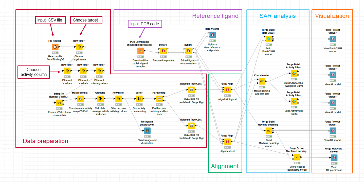
The workflow is divided in 5 blocks which are briefly described below.
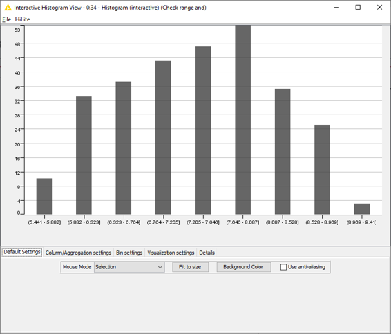
This block of nodes prepares the raw data downloaded from Bindingdb (in this case, from the US9321756 patent: ‘Azole compounds as PIM inhibitors’) for the SAR analysis. Nodes which require manual input are labelled in Figure 1. I need to specify the name and location of the csv file I want to use; choose the biological target I am interested in (US9321756 reports activity for two biological targets – ‘PIM’ and ‘PIM-1’: I used PIM-1) and make sure I am working with the correct activity column (IC50, for PIM-1). There are also nodes to filter away IC50 missing values and those with ‘higher than’ (>) or ‘lower than (<) modifiers, which transform the activity values into pIC50, calculate mean pIC50 values for compounds which were tested multiple times on PIM-1, and remove those compounds where the mean pIC50 is associated with a high standard deviation (>0.7). Finally, the compounds are sorted in order of descending activity to enable an activity stratified partitioning in a training and test set. The ‘Histogram’ node (at the bottom in Figure 1) can be used to check that the distribution and range of the activity values meet the conditions for building robust qualitative and/or quantitative SAR models in Forge. In this case (Figure 2), the activity range covers almost 4 log units and the distribution is reasonably even, so I can confidently go ahead with the model building.
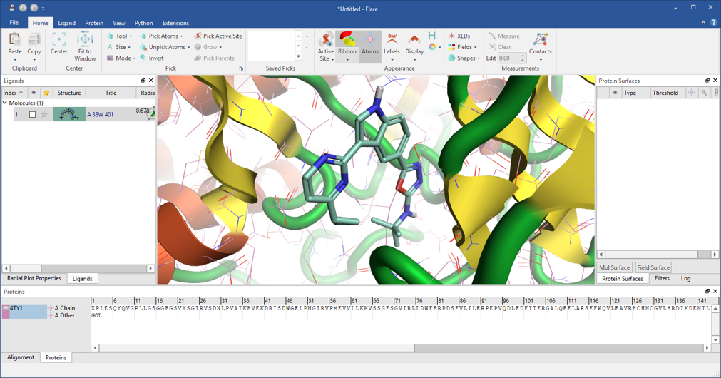
This bit of the workflow downloads the protein-ligand complex with PDB code: 4TY1 and sends it to the new ‘pyflare’ node to prepare the protein, extract the reference ligand, and remove the crystallographic water molecules. The pyflare node allows the Flare Python API to be used from within KNIME, enabling access to all the Flare functionality. The ‘Flare Viewer’ node, also new in this release, can be used to launch Flare and visualize the results, as shown in Figure 3.
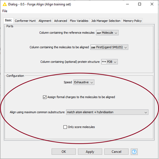
Here I used the ‘Forge Align’ node to align the molecules in the training and test sets to the 38W reference ligand from PDB: 4TY1, using the protein as an excluded volume. I configured the node to use the ‘Exhaustive’ setting (which runs a more accurate conformation hunt), to assign formal charges to the molecules according to the Cresset rules, and to align the molecules by Maximum Common Substructure (MCS), as shown in Figure 4. To speed up the alignment process, I configured KNIME to use the Cresset Engine Broker.
In this final part of the workflow, qualitative and quantitative SAR models are calculated using the ‘Forge Build Field QSAR’, ‘Forge Build Activity Atlas’ and the new ‘Forge Build Machine Learning’ nodes. The visualization is mainly done using the ‘Forge Project Viewer’ node, but as an alternative I could use the ‘Forge Project Writer’ node to save the results into separate project files to view at a later stage.
The Field QSAR method uses Forge 3D electrostatic (based on Cresset’s XED force field) and volume descriptors to create an equation that describes activity, using Partial Least Squares (PLS) analysis. For this case study, I configured the ‘Forge Build Field QSAR’ node to use the ‘Weight molecules by similarity’ option, as shown in Figure 5 - left, which weighs each molecule according to its similarity to the reference. Using this setting will downweigh the importance of training set molecules not optimally aligned to the reference (and accordingly associated with a lower similarity), and may generate better models in those cases where the alignment is not carefully curated. The Field QSAR model shows a Q2 (training set CV, LOO) = 0.52 and a R2 (test set) = 0.65. Visual inspection of the training and test sets and inspection of the PCA plot (Figure 5 – right) reveal that there is a group of compounds with an incorrect protonation state on the pyridine ring. Recalculating the model after removing these compounds from the training and test sets gives a model with similar statistics (Q2 training set CV, LOO = 0.57 and R2 test set = 0.58).
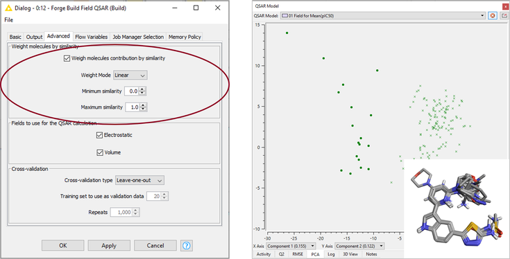
This is a reasonably good starting model which can possibly be improved by further curation of the protonation state and alignment of specific compounds.
The new ‘Forge Build Machine Learning’ node can be used to generate Machine Learning (ML) regression or classification models in KNIME, using Forge 3D electrostatic and volume descriptors. You can decide which model type will be generated (choosing from k-Nearest Neighbors, Random Forest, Relevance Vector Machine or Support Vector Machine), but for this case study I kept the default ‘Auto’ option, which automatically runs all the ML models and pick the best one for the output. To calculate the predicted pIC50 values for the molecules in the test set, I used the new ‘Forge Score Machine Learning’ node. The best performance is obtained with a Support Vector Machine model showing a Q2 (training set CV) = 0.62 and a R2 (test set) = 0.71. Also in this case, recalculating the model excluding the molecules with an incorrect protonation in the pyridine ring from the training and test sets gives a model with similar statistics (Q2 training set CV = 0.57 and R2 test set= 0.69). For this data set, the SVM model is marginally more predictive than the Field QSAR model.
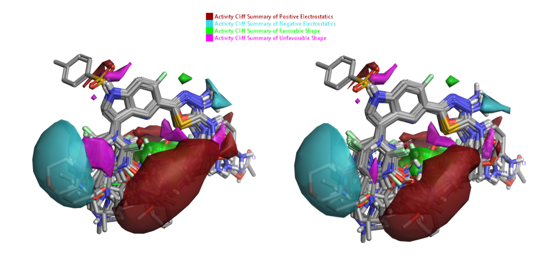
Activity Atlas™ models generate a simple, qualitative picture of the critical points in the SAR landscape. In particular, the ‘Activity Cliff Summary’ views highlight regions of acute SAR and are a useful starting point to understand the data. The new default ‘Weighted Sum’ Activity Cliffs Summary algorithm in the ‘Forge Build Activity Atlas’ node generates more detailed SAR maps by reducing the reliance on individual compounds, and is especially useful for small and medium sized data sets. As this dataset is relatively large though, I also built an alternative Activity Atlas model using the original ‘Sum’ algorithm, which instead focuses on the prevalent SAR signals, and I compared the maps obtained with the two methods. Default conditions were used for all the other options. The two models are shown side by side in Figure 6, and for this case study give very similar results, comparable to those of the original blog post.
V2.5 Cresset KNIME nodes also include additional new features and improvements:
The KNIME workflow built for this post can quickly run a preliminary qualitative and quantitative SAR analysis of any interesting patent data in Bindingdb in an automated manner requiring minimal human intervention. For the US9321756, running this workflow took approximately 30 minutes and resulted in a SVM quantitative SAR model with reasonable predictive ability and clear SAR maps for Activity Atlas. Cresset customers can contact support to get these new components free of charge. Request a free evaluation to try the software yourself.