The adaptability of pyFlare to access advanced data visualization and calculation functionalities
We showcase some examples within a drug discovery context where the pyFlare environment has been further expanded with advanced data ...
News
This sneak peek explores some additional new features in the upcoming release of Flare™, our ligand-based and structure-based platform for drug design.
The identification of potential druggable binding sites for small molecule ligands is a key step in the molecular modeling of novel targets and lead series.
Flare V6 features a new pocket detection module based on fpocket1, a fast protein pocket detection algorithm for the identification and characterization of pockets and cavities within a protein structure, or on its surface.
The pocket detection method works by filling up all potential binding pockets and cavities in a protein structure with ‘alpha-spheres’ of variable size: these are spheres that touch four atoms in the 3D space without containing any internal atoms. The most interesting regions where a binding site could be located, such as for example clefts in the protein surface, typically have a larger occurrence of alpha-spheres. The next step is then to look for sufficiently large clusters of alpha-spheres of proper radius. Fine-tuning the minimum/maximum radius of the alpha-spheres, the minimum number of spheres which populate a pocket, and the maximum size of the cluster makes it possible to search for different types of pockets, for example drug binding sites, water binding pockets, channels and large solvent-exposed sites. The clusters of alpha-spheres can be further characterized according to the properties of the atoms surrounding the spheres (for example, hydrophobicity) to help the identification of druggable binding sites.
Figure 1 shows the results of a pocket detection experiment ran on the apo structure of KEAP1 (PDB: 4IFJ), the key regulator of the NRF2-mediated cytoprotective response, which is an increasingly recognized target for diseases involving oxidative stress.
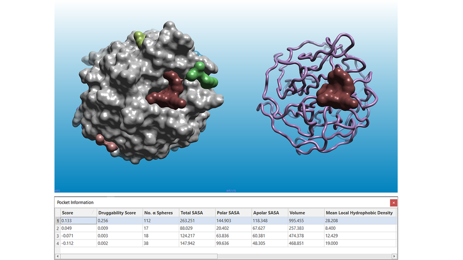
Figure 1. Results of a pocket detection experiment ran on the apo structure of KEAP1 (PDB: 4IFJ). Left: the solvent excluded surface of the KEAP1 protein is shown in grey. Right: the KEAP1 protein structure is shown as a pink ribbon. In both pictures, pockets are shown as multi-color surfaces. The pocket information table (bottom) reports the characterization of the pockets according to a number of different parameters.
The pocket with the highest Score and Druggability Score (brown in Figure 1 and 2) is the binding site of both the NRF2 peptide (PDB: 4IFL, Figure 2 - left) and of small molecule inhibitors2 such as the ligand in PDB: 5FNU (Figure 2 - right).
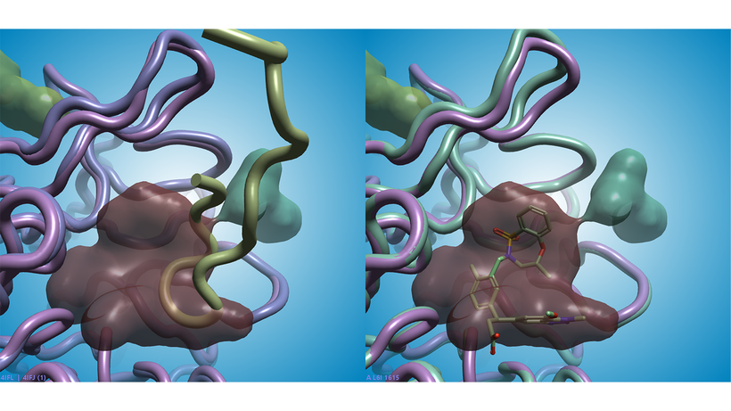
Figure 2. The brown pocket found in PDB: 4IFJ (apo KEAP1 protein: pink ribbon, left and right) has the highest Score and Druggability Score. Left: the brown pocket matches the binding site of the NRF2 peptide in PDB: 4IFL (NFR2 peptide: green ribbon; KEAP1 protein: mauve ribbon). Right: the nanomolar small molecule inhibitor in PDB: 5FNU binds in the same region (ligand: green sticks; KEAP1 protein: green ribbon).
Flare V6 features a new module for running Quantum Mechanics (QM) calculations on ligands, based on the psi43 implementation. This enables you to perform geometry optimizations (minimizations) and/or single point energy calculations of individual ligands, conformation ensembles and ligand poses.
As you choose one of the calculation options, Flare opens a configuration panel where you can choose the desired settings (Figure 3 - left). For each QM method available (HF, MP2 and DFT), a large choice of basis sets is available (Figure 3 -right). The single point energy calculation can be performed in vacuum, water or a number of organic solvents. Calculations are multi-threaded, and you can connect Flare to the Cresset Engine Broker™ to access remote calculation resources and significantly reduce the overall calculation time.
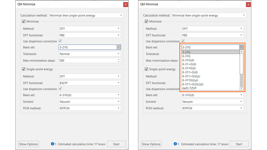
Figure 3. The QM minimization and single-point energy calculation panel in Flare.
The choice of options for the default methods gives the best trade-off between reasonable speed and accuracy of results. Information, warning and error messages at the bottom of the calculation panel help you understand whether your calculation is set-up correctly before pressing the ‘Start’ button.
QM calculations in Flare also include the computation of the molecular electrostatic potential for ligands, ligand conformations and ligand poses (Figure 4).
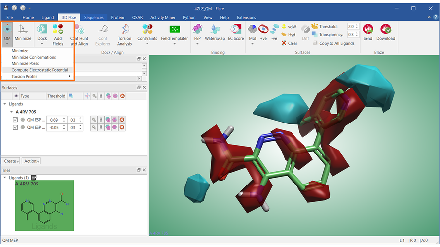
Figure 4. QM molecular electrostatic potential for the ligand in PDB: 4ZLZ. Cyan: negative electrostatic potential; Red: positive electrostatic potential.
QM torsion profiles for selected rotamers in ligands of interest (Figure 5) can be calculated using a wizard and stored locally for future reference.
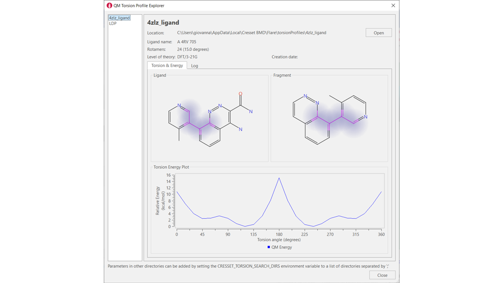
Figure 5: QM torsion profile for the highlighted torsion of the PDB: 4ZLZ ligand.
Running calculations from the command-line using the pyflare binary is invaluable whenever you think big - for example if you are considering docking or aligning tens of thousands of ligands, or if you wish to run long Dynamics or Free Energy Perturbation calculations without opening the Flare GUI.
In Flare V6, we have made it simpler to run your command-line experiments, making the most of the Flare user-friendly GUI in the set-up, and of the power of pyflare and the Cresset Engine Broker in the execution.
For example, let’s say you want to run a large docking calculation. You can set-up your calculation as usual in the Flare GUI, choosing all the desired options: for example, setting the docking grid and choosing the protein and protein chains to use, and whether to use a quick, normal or accurate calculation method (Figure 6).
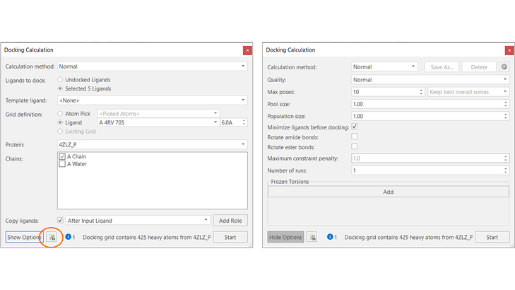
Figure 6. Use the Flare docking calculation panel (left) and the docking advanced options (right) to set-up the docking experiment. Press the ‘Export’ button to save all the required information to run the experiment from the command-line.
Pressing the ‘Export’ button at the bottom of the calculation panel will then save all the files and information required for running the experiment from the command-line in a directory of your choice (Figure 7). If you have configured Flare to use the Cresset Engine Broker to access remote calculation resources, the script will automatically use it.
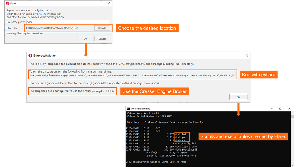
Figure 7. Flare will save all required files and information in the chosen directory, with clear instructions on how to run the experiment.
You are now ready to start the docking experiment by either using pyflare with the ‘dock.py’ Python script created by Flare, or, if you are working on Windows/Linux, by using the ‘dock.bat’/’dock.sh’ executables.
Flare V6 will be launched this summer.