Improving PROTAC properties via single-point changes to linkers
We explore how computational methods can be applied to proteolysis targeting chimera (PROTAC) design, to effectively tackle some of the ...
News
Free Energy Perturbation (FEP) calculations arm the drug hunter with highly accurate binding affinity predictions for ligands. This accuracy can be better than 1 kcal/mol from experimental values, so can make a significant difference in successfully selecting the molecules with the most potential for further development and synthesis. However, common barriers to using FEP are typically that the calculations are very involved, i.e., difficult to setup and execute, and can also take a long time to run. Therefore, FEP can have the reputation to be expensive in terms of both user and total computational time. Flare FEP, a component of the Flare ligand and structure-based design platform, significantly lowers this barrier as very accurate FEP results are found quickly and easily. Below I describe the speed, accuracy, and ease of use which research chemists can expect from Flare FEP, which is available for evaluation on request.
The recent release of Flare V5 offers a significant improvement in the speed of Flare FEP simulations. Calculations in Flare V5 are now, for medium sized systems, at least 2.5-3.5x faster than Flare V4. For the ‘TYK2’ example from the Wang et al benchmark sets, (including 11 ligands, 14 links and 28 perturbations) this equates to 106 GPU hours in Flare V5 versus 470 GPU hours in Flare V4. In ‘real time’, if you have a 10 GPU cluster (Flare FEP calculations require GPUs which support OpenCL or NVIDIA CUDA), this is equivalent to about 10.6 hours for 11 molecules versus  47 hours, which makes a vast improvement for the time it takes to see results.

Figure 1. Tooltip pop-up for Flare FEP calculations. Compare total GPU hours for Flare V5 (left) versus Flare V4 (right) for a TYK2 Flare FEP benchmark run. Number of ligands, links and perturbations remain the same for this example, but the difference in Lambda windows allows for a >4x speedup.
A combination of improvements that have enabled this fast FEP run-time are discussed below. Most obviously from this example, the change in Lambda assignments has been a big improvement.
Lambda windows between perturbations represent the incremental jumps made as the ligand is transformed from A to B. It can be non-obvious and time-consuming to set the Lambda windows manually, and setting a blanket default number can be wasteful when some perturbations are trickier than others.
If you were to decide the Lambda windows for each link yourself (of which there may be hundreds) you cannot know ahead of the calculation if you are over or underestimating the Lambda windows. If you under-sample and there is insufficient overlap between Lambdas the results need to be discarded and re-run (Figure 2 - left). If you over-sample with more than the required Lambda windows, more than sufficient overlap is reached at the cost of a more expensive calculation (Figure 2 - middle). Unless you choose exactly right, either way is wasteful in terms of calculation time.

Figure 2. Compares under-sampling (9 Lambda windows, left) versus over-sampling (21 Lambda windows, middle) versus the adaptive Lambda scheduling (12 Lambda windows, right) for the link between 20~1h1q in one of the benchmarks CDK2.
These issues are removed with the new ‘adaptive Lambda scheduling’ where a fast (50ps) pre-calculation at the start of the FEP run determines the optimal number of Lambda windows required for each particular perturbation, so you don’t have to (Figure 2 – right).
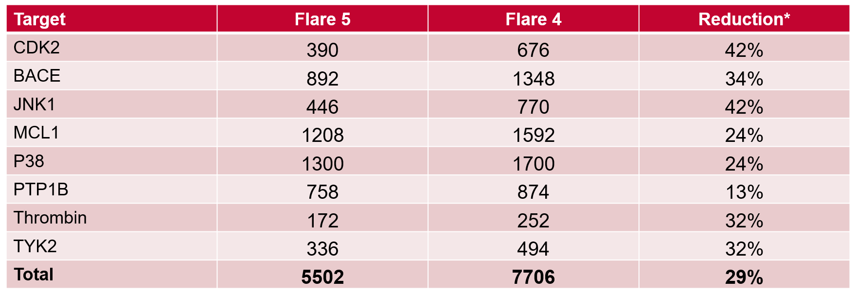
Table 1. Number of total Lambda windows required in Flare V5 vs. V4, and % reduction. *Assuming no links needed to be re-run with more Lambda windows.
For the 8 data sets in the Wang benchmark, significantly fewer total Lambda windows are required using the adaptive Lambda sampling in Flare V5, versus choosing a fixed set of 9 Lambda windows for every link in Flare V4 (Table 1). In fact, the ~30% fewer calculations is an under-estimate, given it does not count any calculation that is discarded due to under-sampling (Figure 2 - left), or if more calculations are done than are required in over-sampling (Figure 2 – middle).
We have changed the integrator used in the Flare FEP dynamics calculations. The new LangevinMiddleIntegrator is more stable and allows for a longer timestep to be used. By adding a small amount of Hydrogen Mass Repartitioning (HMR), in which the hydrogen masses are repartitioned according to the heavy atom it is attached to without changing the overall total mass, we have been able to increase the default timestep from 2fs to 4fs with no loss of stability. This provides a nearly twofold decrease in the required GPU time per link.
A truncated octahedral water box is another development implemented in the MD stage, which reduces the time of the Flare FEP calculation. The octahedral shape is a more efficient unit cell in MD as it approximates more closely a sphere. This reduces the amount of water molecules required in the simulation and accordingly the length of the simulation. For a small example protein, using an octahedral box for the simulation cell decreased the number of atoms from 17.5K to 10K atoms with respect to using a cubic box (Figure 3). Testing has also shown that a smaller water box buffer of 6Å in Flare V5 (versus 10Å in Flare V4) is sufficient to simulate an isolated  protein-ligand complex in solution (without interactions between nearby cells).
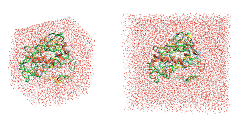
Figure 3. New truncated octahedral water box in Flare V5 (left) reduces the number of atoms included in the MD simulation (10K atoms) with respect to the cubic water box right, (17.5K atoms) used in Flare V4.
In Flare V5 we have made a number of improvements under the hood to allow FEP calculations to be run on larger data sets. If you have many molecules, then the calculations to set up the perturbation network (i.e., which molecule pairs are chosen to run perturbation calculations on) can take a significant amount of time. The new code not only makes these calculations much faster, but also enables parallelization across multiple CPU cores and over multiple machines. As a result, standard perturbation graphs can easily be generated for data sets of ~150 ligands and Star graphs can be set up for 500 or more ligands (Figure 4).
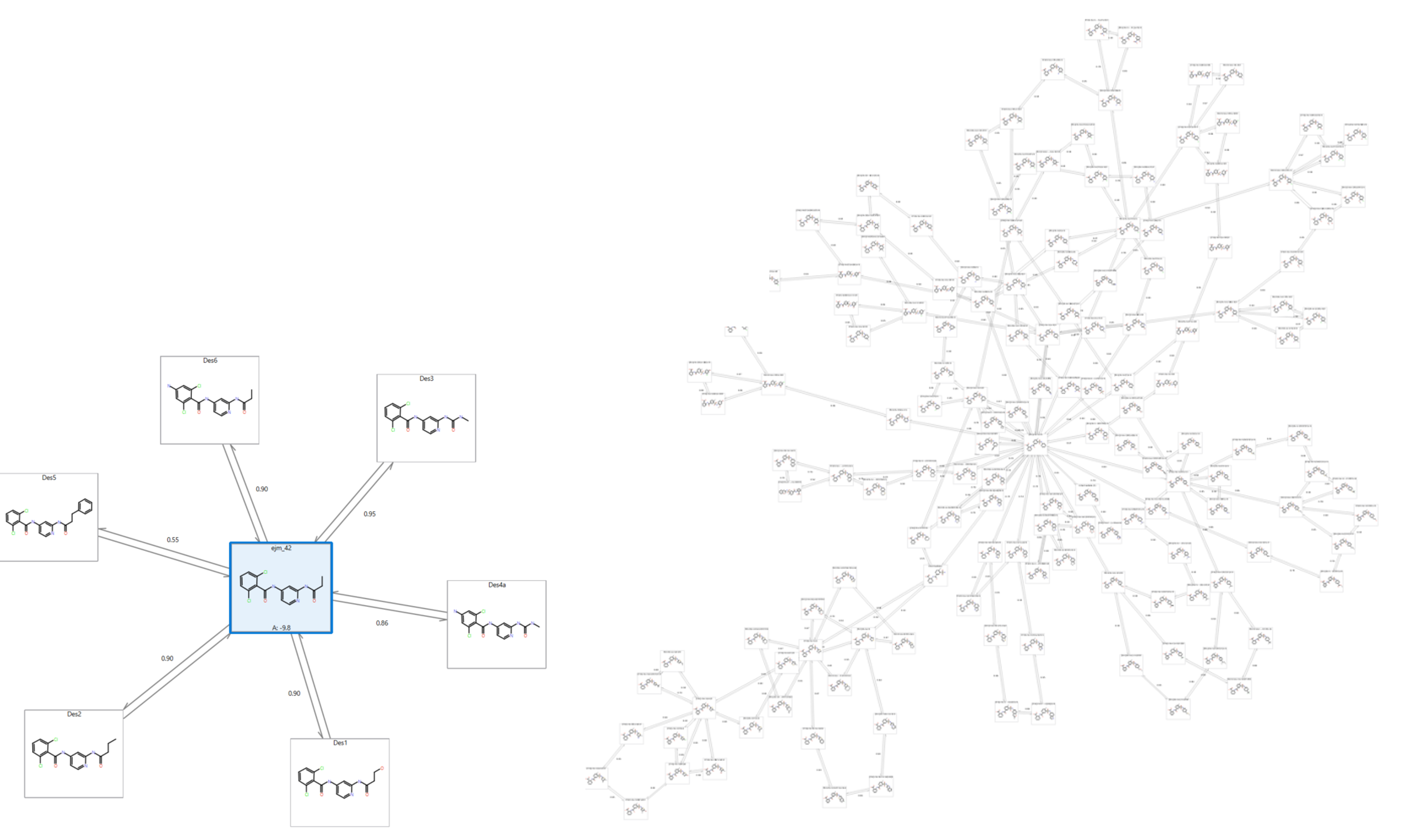
Figure 4. Comparison of a Star graph (left) and a Normal perturbation graph (right) of ~150 ligands. Star graphs can accommodate up to 500 ligands, but a smaller example is shown here for clarity.
Working at this scale enables you to quickly focus on the molecules worth pursuing. For example, a Spark™ experiment which produces 500 results can be analyzed in a quick mode, Star graph Flare FEP experiment, further refining the most promising results (say 50 from the original 500) using a dual linked, Normal graph. This enables you to triage quickly for the best molecules and ultimately prioritize with robust and accurate binding free energy predictions a much smaller subset of molecules to be confidently synthesized and tested.
Most importantly, the speed improvements in Flare V5 do not affect the predictive performance and accuracy of Flare FEP. Flare V5 still delivers robust results, as previously demonstrated in Assessment of Binding Affinity via Alchemical Free Energy Calculations J. Chem. Inf. Model. 2020. Mean Unsigned Error (MUE) values calculated with Flare FEP using the method ‘out of the box’ compare favorably with those previously obtained, with all but one example showing a MUE <1 kcal/mol (Figure 5).
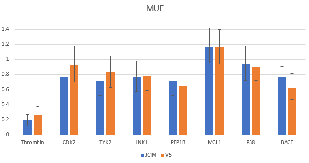
Figure 5. MUE comparing previously published data from Kuhn et al (in blue) and latest results using the new release of Flare V5 (in orange) for the Wang et al benchmark data set.
The Custom Force Field Wizard enables you to easily select the torsion of interest and edit the molecule to reduce the atoms not required to get a good parameterization of the torsion. The drop-down list of various Quantum Mechanics methods and basis sets enables you to create a tailored parameterization to supplement AMBER GAFF or GAFF2.
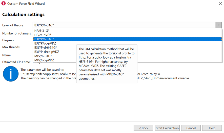
Figure 6. The Custom Force Field Wizard presents a variety of QM methods and basis sets for adding custom torsional parameters to your ligand data set using GAFF and GAFF2.
In addition to the vast improvements in Flare FEP run-time, there are also enhancements which enable easier and more efficient process in setting up the FEP simulation. These developments are seen in the generation of the perturbation network graph.
Link scores between perturbations (Figure 7) inform you of the ease of which the ligand A will transform to B. This is on a scale of 0 (very dissimilar) to 1 (identical).
For some ligands, very low link scores (e.g., <0.4) are not going to produce good results. In this case, it is recommended an ‘intermediate‘ structure is added to facilitate the A⇒B transition and improve your results. Adding intermediate structures manually is cumbersome: you have to design, edit and align your molecule to your original set, and you may have to do this many times depending on the size and details of the ligand data set. Automating this process vastly improves usability: Cresset’s new rule-based heuristic algorithm creates intermediates where needed and  where they will work well in improving the Flare FEP simulation.
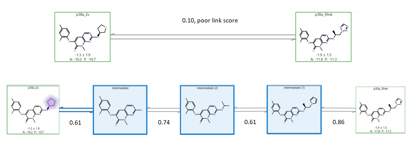
Figure 7. Demonstrating the intermediate generation process. The two known molecules in the green boxes have a poor link score (0.10) without intermediates (they are very dissimilar). Adding intermediates (blue boxes) until the link scores exceed 0.6 much improves the quality of the results without requiring any user intervention.
Using Flare FEP ‘out of the box’ (Figure 5), usually gives fast and very good initial results. Once you have carefully prepared and set up your protein target, only minutes are required to generate the initial perturbation network and start the Flare FEP calculation.
Sanity checking the perturbation map pre-calculation, and possibly making refinements post-calculations, may further increase the accuracy of the results.
The user-friendly Flare FEP interface facilitates the inspection and further refinement of the initial results. It makes all the important go-to areas for sanity checking your project visible: the 3D structures of equilibrated ligands, the quality of the overlap matrices, the cycle closure errors, the links in the log to any potential issue, and the Activity Plot.
The 1 minute web clip ‘Easy analysis of Flare FEP results’ demonstrates the ease of analysis and refining of results in Flare FEP. Note the Activity Plot with statistics and a synchronization between the data points and the ligands which you can visualize in 3D to examine protein and water interactions. As in this example, if there is a ‘poor overlap’ you can examine this in the Overlap Matrix tab to see if there are windows that could be improved with a quick revision of the link.
You also have the power to manually tweak and delete intermediates if they are thought unnecessary. However, generally the algorithm gives the right amount of molecules to improve the accuracy versus taking a large transformation step in one go. There is also now the option to force the re-equilibration of a ligand without clearing any completed links, and push back the equilibrated complex to Flare for analysis in 3D. All these developments help ease the  troubleshooting and refinement of your FEP results to deliver predictions you have confidence in.
See the flexible licensing options for Flare and request an evaluation to try it on your project.